Geospatial Data Processing with GeoPandas in Python
Process geospatial data in Python with GeoPandas: read vector files, work with Shapely geometries, run spatial operations, and manage coordinate reference systems.
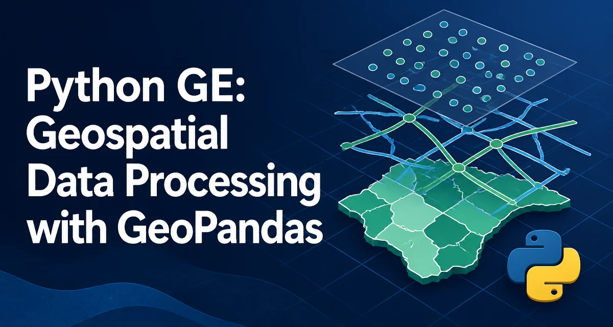
GeoPandas is a popular Python library for working with vector geospatial data. It extends pandas with a dedicated geometry column, so you can keep attributes and geometries together and use familiar DataFrame operations for filtering, grouping, and analysis. The actual geometry objects come from Shapely, and GeoPandas handles file I/O for common vector formats such as shapefiles and GeoJSON.
This article explains the practical essentials: reading and writing vector files, creating and manipulating geometries, performing spatial operations, and managing coordinate reference systems (CRS). It also covers common performance and data-quality pitfalls.
Core Libraries for Geospatial Work
The main pieces of this ecosystem are:
- GeoPandas: Extends pandas with GeoDataFrame and GeoSeries classes and adds spatial methods to geometry columns.
- Shapely: Provides geometric primitives such as Point, LineString, Polygon, and Multi-part versions, plus operations like buffer, intersection, and union.
- Fiona: An OGR-based I/O library for reading and writing vector formats.
- Pyproj: Handles coordinate transformations and geodetic calculations.
| Library | Purpose |
|---|---|
| GeoPandas | High-level dataframe operations with geometry columns |
| Shapely | Low-level geometry creation and analysis |
| Fiona | File I/O for vector formats |
| Pyproj | Coordinate reference system transformations |
In day-to-day work, GeoPandas calls into Shapely and the vector I/O layer for you. Knowing each library still helps when you need lower-level control over geometry operations or file format options.
Reading and Writing Geospatial Data
Use read_file to read a vector dataset:
import geopandas as gpd

gdf = gpd.read_file('path/to/file.shp')
The result is a GeoDataFrame with attribute columns and a geometry column. The geometry column contains Shapely geometries, and the crs attribute records the coordinate reference system of the file, if the file specifies one.
Writing to GeoJSON is equally straightforward:
gdf.to_file('output.geojson', driver='GeoJSON')
The driver parameter tells the I/O backend which format to use. For a shapefile, use driver='ESRI Shapefile'. In many cases GeoPandas can also infer the driver from the file extension.
Working with Geometries
Shapely provides the main geometry types: Point, LineString, Polygon, and their Multi counterparts. GeoPandas stores these objects in a geometry column.
Create a point like this:
from shapely.geometry import Point

point = Point(12.5, 41.9)
You can measure the distance between two geometries:
other_point = Point(12.6, 41.8)
distance = point.distance(other_point)
For a geographic CRS such as EPSG:4326, this distance is in degrees, not meters or miles. Shapely performs planar calculations, so for accurate ground distances you should reproject to an appropriate projected CRS or use a geodetic computation library.
Spatial Operations and Analysis
Spatial operations let you answer questions about proximity, overlap, and containment. Common operations include buffer, intersection, union, and difference.
For example, create a buffer around a point and find polygons that intersect it:
buffered = point.buffer(0.01)
intersecting = gdf[gdf.geometry.intersects(buffered)]
gdf.geometry.intersects(buffered) returns a boolean Series, one value per row, indicating whether that row's geometry intersects the buffered point. It can then be used to filter the GeoDataFrame.
These operations use Shapely under the hood, but GeoPandas gives them a DataFrame-friendly interface.
Handling Coordinate Reference Systems
A coordinate reference system (CRS) defines how coordinate values correspond to locations on the Earth. If two datasets use different CRSs, their geometries will not line up correctly.
GeoPandas stores CRS information in the crs attribute. Use to_crs to reproject to a different CRS:
gdf_web_mercator = gdf.to_crs('EPSG:3857')
EPSG codes are standard identifiers for CRSs. Common examples are EPSG:4326 (WGS84 latitude/longitude) and EPSG:3857 (Web Mercator). Before combining datasets, check gdf.crs on each one and reproject when necessary.
Performance and Memory Considerations
Vector datasets can grow large enough that reading and processing them in memory becomes expensive. A spatial index speeds up spatial joins and bounding-box queries. GeoPandas provides an R-tree spatial index through the sindex attribute:
spatial_index = gdf.sindex
GeoPandas uses this index internally for spatial joins; you can also query it to find candidate geometries for intersection tests.
For very large datasets, consider streaming features with Fiona's fiona.open iterator, or move the data into a spatially enabled database such as PostGIS.
Common Pitfalls and How to Avoid Them
- CRS mismatches: Always check
gdf.crsbefore combining datasets. - Invalid geometries: Use
gdf.is_validto detect invalid geometries;gdf.buffer(0)can repair some of them. - Large file I/O: Stream features when possible instead of loading the whole file into memory.
- Distance and area units: Planar distance and area calculations are meaningful only in a projected CRS. For geographic coordinates, use projection or a geodesic method.
By keeping these points in mind, you can avoid silent errors that produce incorrect spatial results.