Python SciPy Sparse Matrices and Linear Algebra

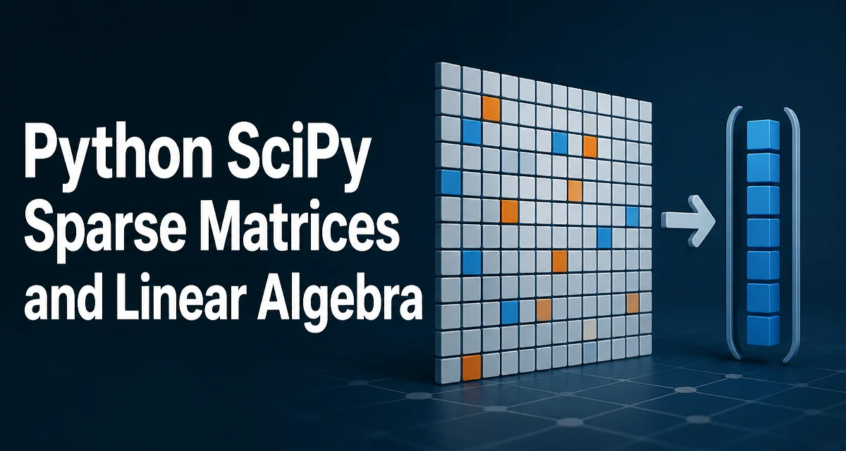
Python SciPy sparse matrices and linear algebra are essential tools when your data is large and mostly zeros. This guide covers creating sparse matrices, performing operations, and solving linear systems efficiently with scipy.sparse and scipy.sparse.linalg.

Why Sparse Matrices Matter

Many real-world datasets—graph adjacency matrices, finite-element meshes, recommendation systems—are sparse: most entries are zero. Storing them as dense NumPy arrays wastes memory and compute. For example, a 100,000 x 100,000 matrix with 0.1% nonzeros would consume ~80 GB as float64, but only ~80 MB in a sparse format. Sparse structures store only nonzero values and their positions, enabling operations that scale with the number of nonzeros rather than the full dimensions.

SciPy provides a family of sparse matrix classes in scipy.sparse, each with different strengths. The choice of format directly affects performance of arithmetic, slicing, and conversions.

Creating Sparse Matrices

The simplest way to create a sparse matrix is from a dense NumPy array using csr_matrix or coo_matrix:

import numpy as np
from scipy.sparse import csr_matrix, coo_matrix

dense = np.array([[0, 0, 1], [2, 0, 0], [0, 3, 0]])
sparse_csr = csr_matrix(dense)
print(sparse_csr)

Output:

  (0, 2)	1
  (1, 0)	2
  (2, 1)	3

For large matrices, constructing from coordinate lists avoids building a dense array. Use coo_matrix with row, column, and data arrays:

rows = [0, 1, 2]
cols = [2, 0, 1]
data = [1, 2, 3]
sparse_coo = coo_matrix((data, (rows, cols)), shape=(3, 3))

COO is efficient for assembly but not for arithmetic. Convert to CSR or CSC before operations:

sparse_csr = sparse_coo.tocsr()

Choosing the Right Sparse Format

SciPy offers several formats, each optimized for different tasks. The most common are:

For most linear algebra, csr_matrix is the default choice because it supports efficient matrix-vector multiplication and is the input format for spsolve. If you need to modify entries frequently, start with lil_matrix and convert to csr when done.

Basic Linear Algebra Operations

Sparse matrices support the same arithmetic operators as dense arrays, but with different performance characteristics.

Matrix-vector multiplication is fast and uses the sparsity structure:

v = np.array([1, 2, 3])
result = sparse_csr.dot(v)  # or sparse_csr @ v

Matrix-matrix multiplication works as expected, but the result may become denser. SciPy automatically selects an efficient algorithm for CSR-CSR products:

product = sparse_csr @ sparse_csr.T

Element-wise operations like addition and subtraction are also supported, but the result's sparsity pattern is the union of the operands. If both matrices are large and sparse, the result may have many more nonzeros.

Solving Linear Systems

The scipy.sparse.linalg module provides spsolve for direct solving of sparse linear systems. It uses LU decomposition and works well for moderate-sized matrices (up to tens of thousands of unknowns).

from scipy.sparse import csr_matrix
from scipy.sparse.linalg import spsolve

A = csr_matrix([[4, 1, 0], [1, 3, 1], [0, 1, 2]])
b = np.array([1, 2, 3])
x = spsolve(A, b)

spsolve requires A to be in CSR or CSC format and returns a dense array. For symmetric positive-definite matrices, scipy.sparse.linalg.spsolve with use_umfpack=True (if installed) can be faster, but the default is robust.

For very large systems, iterative solvers like cg (conjugate gradient) or gmres are more memory-efficient. These are available in scipy.sparse.linalg and accept a linear operator or sparse matrix:

from scipy.sparse.linalg import cg
x, info = cg(A, b, tol=1e-6)

Eigenvalue Problems

Finding eigenvalues of sparse matrices is common in physics and graph analysis. scipy.sparse.linalg.eigs computes a few eigenvalues for general matrices, while eigsh is optimized for symmetric matrices.

from scipy.sparse.linalg import eigsh

# A is a sparse symmetric matrix
eigenvalues, eigenvectors = eigsh(A, k=3, which='SM')

eigsh uses ARPACK and requires a symmetric matrix. For non-symmetric matrices, use eigs. The k parameter specifies how many eigenvalues to compute; which selects the smallest ('SM') or largest ('LM') magnitude.

These functions work with CSR or CSC input and are far more memory-efficient than numpy.linalg.eig, which would densify the matrix.

Performance and Memory Considerations

The main benefit of sparse matrices is reduced memory usage and faster operations when the sparsity is high. However, certain operations can be unexpectedly expensive:

• Converting between formats (e.g., csr to csc) requires a sort and can be O(nnz log nnz).
• Slicing a CSR matrix by rows is efficient, but slicing by columns is slow. Use CSC for column slicing.
• Element-wise operations that produce dense results (like adding two matrices with disjoint sparsity patterns) can blow up memory.
• Matrix-vector multiplication is O(nnz) and very fast, but matrix-matrix multiplication can produce a dense result if the sparsity pattern is unfavorable.

Always check the number of nonzeros after operations using .nnz to avoid accidental densification.

Common Pitfalls and Best Practices

A frequent mistake is converting a sparse matrix to a dense array with .toarray() just to inspect it. For large matrices this defeats the purpose. Use print(A) or A.nnz instead.

Another issue is using np.linalg.solve on a sparse matrix; it will silently densify the input. Always use spsolve or iterative solvers.

When building a sparse matrix incrementally, avoid repeatedly inserting into a csr_matrix. Use lil_matrix or coo_matrix for assembly and convert once.

Finally, be mindful of the data type. Sparse matrices default to float64. If your data is integer or boolean, you may need to cast explicitly to avoid unexpected type promotion in operations.

By understanding the formats and the available linear algebra routines, you can handle large-scale problems that would be impossible with dense arrays.