Python Sentence Transformers: Cosine Similarity and Semantic Search
Learn how to use Python sentence transformers and cosine similarity to build semantic search. Covers model loading, embeddings, similarity scoring, vector indexes, and practical trade-offs.
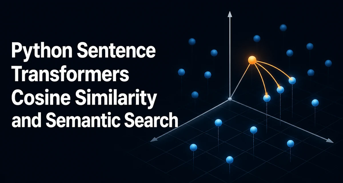
This guide shows how to use Python sentence transformers to compute cosine similarity between sentence embeddings and build a semantic search pipeline. A keyword search finds texts that contain the same words, but semantic search finds texts that mean the same thing. Sentence transformers map text to dense vectors, and cosine similarity measures how close those vectors are.
What Sentence Transformers Provide for Semantic Search
Sentence transformers are pre-trained neural network models that convert a sentence or short paragraph into a fixed-size vector. These vectors live in a high-dimensional space where semantic similarity corresponds to geometric proximity. Two sentences with similar meaning produce vectors that are close together, even if they share no vocabulary.
For semantic search, you encode every document in your corpus into an embedding and store those vectors. When a query arrives, you encode it the same way and find the stored vectors closest to the query vector. Cosine similarity is the standard distance metric because it measures the angle between vectors, ignoring their magnitude. This is important because sentence transformers do not normalize embeddings by default, and vector length can vary with sentence length and style.
The sentence-transformers library provides a consistent API for loading models, encoding texts, and comparing results. It is built on PyTorch and includes many pre-trained models tuned for semantic similarity, retrieval, and clustering.
Installing and Loading a Sentence Transformer Model
The library installs with pip and pulls in the necessary dependencies, including PyTorch.
pip install sentence-transformers
After installation, loading a model is a single call. The library downloads the model weights on first use and caches them locally.
from sentence_transformers import SentenceTransformer

model = SentenceTransformer('all-MiniLM-L6-v2')
The model identifier points to a pre-trained model on the Hugging Face Hub. all-MiniLM-L6-v2 is a compact model that balances speed and quality for many use cases. It produces 384-dimensional embeddings and works well for English text. For multilingual scenarios, models like paraphrase-multilingual-MiniLM-L12-v2 are available.
Encoding Sentences into Embeddings
The core method is encode(). It accepts a single string or a list of strings and returns a NumPy array (or a PyTorch tensor, depending on the output format).
sentences = [
    "The cat sat on the mat.",
    "A feline rested on the rug.",
    "The stock market rose sharply today."
]

embeddings = model.encode(sentences)
print(embeddings.shape)  # (3, 384)
Each row corresponds to one sentence. The model applies tokenization, padding, and pooling internally, so you do not need to preprocess the text manually. You can pass device='cuda' to run encoding on a GPU when one is available.
embeddings = model.encode(sentences, device='cuda')
For large corpora, batch processing is more efficient. The batch_size parameter controls how many sentences are processed at once, and show_progress_bar gives feedback for long-running jobs.
embeddings = model.encode(all_documents, batch_size=64, show_progress_bar=True)
The output is a 2D array where each row is a sentence embedding. These embeddings are not normalized by default, so cosine similarity must account for vector magnitudes.
Computing Cosine Similarity Between Embeddings
Cosine similarity is defined as the dot product of two vectors divided by the product of their magnitudes. In Python, you can compute it directly with NumPy or use scikit-learn's cosine_similarity function.
import numpy as np

def cosine_similarity(a, b):
    return np.dot(a, b) / (np.linalg.norm(a) * np.linalg.norm(b))
For a single query against a corpus, you can compute similarity scores for all documents at once.
query = "A cat was resting on a floor covering"
query_embedding = model.encode(query)

scores = [cosine_similarity(query_embedding, doc_emb) for doc_emb in embeddings]
Alternatively, use scikit-learn's vectorized implementation:
from sklearn.metrics.pairwise import cosine_similarity

scores = cosine_similarity([query_embedding], embeddings)[0]
This returns an array of similarity scores between -1 and 1. Higher scores mean greater semantic similarity. For retrieval, you typically sort by score and take the top-k results.
A common optimization is to normalize all embeddings to unit length before storing them. With normalized vectors, cosine similarity reduces to a simple dot product, which is faster and allows you to use efficient dot-product-based indexes.
normalized_embeddings = embeddings / np.linalg.norm(embeddings, axis=1, keepdims=True)
query_norm = query_embedding / np.linalg.norm(query_embedding)

scores = normalized_embeddings @ query_norm
Building a Semantic Search Pipeline with a Vector Index
For small corpora, computing cosine similarity against every document is acceptable. For thousands or millions of documents, a brute-force scan becomes slow. A vector index organizes embeddings so that nearest-neighbor queries can avoid a full scan; many indexes trade a small amount of recall for much faster search.
FAISS is a popular library for this purpose. It works with normalized embeddings and supports inner-product search, which is equivalent to cosine similarity when vectors are unit length.
import faiss

dimension = normalized_embeddings.shape[1]
index = faiss.IndexFlatIP(dimension)
index.add(normalized_embeddings)
IndexFlatIP performs exact inner-product search. It is fast for moderate sizes and returns exact results. For larger corpora, you can use an inverted file index (IndexIVFFlat) that partitions the space and only searches a subset of clusters.
nlist = 100
quantizer = faiss.IndexFlatIP(dimension)
index = faiss.IndexIVFFlat(quantizer, dimension, nlist)
index.train(normalized_embeddings)
index.add(normalized_embeddings)
When querying, you specify the number of nearest neighbors to retrieve.
distances, indices = index.search(query_norm.reshape(1, -1), k=5)
The returned indices map to rows in your original document list. The distances are the cosine similarity scores (since vectors are normalized).
Other vector databases like Chroma, Qdrant, or Elasticsearch with vector support can serve the same purpose. The choice depends on your deployment requirements: whether you need persistence, filtering, or horizontal scaling.
Performance and Practical Considerations
Encoding is the most expensive step. Throughput depends on the model, batch size, and hardware. GPU acceleration can help when you need to encode queries in real time. For a one-time indexing job, CPU is often sufficient. For real-time query encoding, a GPU or a smaller model may be necessary.
Memory usage scales with the number of embeddings and their dimensionality. A 384-dimensional float32 vector uses about 1.5 KB. A million documents require roughly 1.5 GB of RAM. If that is too much, you can reduce precision to float16 or use product quantization in FAISS, which compresses vectors at the cost of some recall.
When updating the index, consider whether you need incremental additions or a full rebuild. IndexFlatIP supports adding vectors, but IndexIVFFlat requires training before adding. If your corpus changes frequently, a simpler index or a database with built-in vector support may be easier to maintain.
Another practical point: sentence transformers are sensitive to input length. Most models truncate sequences longer than their maximum token limit (often 256 or 512 tokens). For long documents, split them into sentences or paragraphs and index each chunk separately, then aggregate retrieval results at the document level.
Choosing the Right Model and Similarity Metric
Different models produce embeddings with different properties. all-MiniLM-L6-v2 is a good default for English semantic similarity. For domain-specific text, models fine-tuned on that domain often perform better. The Hugging Face Hub includes models trained for scientific papers, legal text, and code.
Cosine similarity is not the only option. Dot product on normalized vectors is equivalent, but Euclidean distance (L2) can also be used. When embeddings are normalized, ranking by L2 distance is inversely related to cosine similarity, so the top results are the same. In practice, cosine similarity is preferred because it is bounded and interpretable.
If your task involves asymmetric retrieval—for example, short queries against long documents—consider models trained for that scenario, such as msmarco-distilbert-base-v4. They are optimized to rank relevant passages for query-style inputs, which can improve retrieval quality compared with symmetric similarity models.
Finally, evaluate the model on your own data. A small validation set of queries with known relevant documents is enough to compare models by retrieval recall. The best model for your domain may not be the most popular one, and the only way to know is to test.